Metagenomics provenance walkthrough

This notebook is a worked example for the FAIR metagenomics workflow described in A metadata-managed FAIR end-to-end workflow for microbial community omics data analysis. It shows, with real data:

• how the published provenance graphs can be queried to find out exactly what was executed — which container, when, and on which inputs;
• how the same records support biological interpretation of the benchmark, e.g. functional predictions across assembly configurations.

Everything below is pre-rendered: the tables and figures were produced by running the SPARQL queries against the deposited RDF graphs (Zenodo record 10.5281/zenodo.17990145). No installation or re-running is needed to read this page; to reproduce the numbers yourself, see the last section.

All numbers come from the deposited graphs — nothing here is synthetic or estimated.

1. What we query

The manuscript’s Methods section (Worked provenance query) contains the following SPARQL query. It retrieves, for every executed workflow step, the process-run identifier, start/end timestamps, the container image, and the compressed input files:

PREFIX prov: <http://www.w3.org/ns/prov#>
PREFIX wfprov: <http://purl.org/wf4ever/wfprov#>
PREFIX wfdesc: <http://purl.org/wf4ever/wfdesc#>
PREFIX cwlprov: <https://w3id.org/cwl/prov#>
PREFIX nsprov: <http://www.w3.org/ns/prov#>
SELECT DISTINCT ?processRun ?startTime ?endTime ?image ?input
WHERE {
  GRAPH ?g {
    ?plan a prov:Plan ; wfdesc:hasSubProcess ?subProcess .
    ?association prov:hadPlan ?subProcess .
    ?processRun prov:qualifiedAssociation ?association ;
                a wfprov:ProcessRun ;
                prov:qualifiedStart/prov:atTime ?startTime ;
                prov:qualifiedEnd/prov:atTime ?endTime ;
                prov:wasAssociatedWith/cwlprov:image ?image .
    OPTIONAL {
      ?processRun prov:qualifiedUsage/nsprov:entity ?entity .
      ?entity cwlprov:basename ?input .
      FILTER(STRENDS(?input, ".gz"))
    }
  }
}

The query was executed against the three public provenance graphs (BMOCK12_PROVENANCE.trig.gz, ZYMO_EVEN_PROVENANCE.trig.gz, ZYMO_LOG_PROVENANCE.trig.gz). The results below are stored alongside this notebook.

%matplotlib inline
import pandas as pd
import matplotlib
import matplotlib.pyplot as plt
from pathlib import Path
import sys

RES = Path("results")
pd.set_option("display.max_colwidth", 120)

print("python", sys.version.split()[0])
print("pandas", pd.__version__)
print("matplotlib", matplotlib.__version__)

worked = {
    name: pd.read_csv(RES / f"{name}_provenance_worked_query.csv")
    for name in ["BMOCK12", "ZYMO_EVEN", "ZYMO_LOG"]
}
full = pd.read_csv(RES / "prov_query_even_flye.csv")
pfam = pd.read_csv(RES / "sapp_query_combined_pfam_accession.csv")
print("loaded", {k: len(v) for k, v in worked.items()})

python 3.13.7
pandas 2.3.2
matplotlib 3.10.7
loaded {'BMOCK12': 3658, 'ZYMO_EVEN': 4434, 'ZYMO_LOG': 2684}

2. Result overview

The query returns one row per executed workflow step. The number of steps recorded per benchmark dataset is:

summary = pd.DataFrame(
    [
        {
            "Dataset": name,
            "Process runs returned": len(df),
            "Distinct container images": df["image"].nunique(),
            "First run": df["startTime"].min()[:10],
            "Last run": df["endTime"].max()[:10],
        }
        for name, df in worked.items()
    ]
)
summary

	Dataset	Process runs returned	Distinct container images	First run	Last run
0	BMOCK12	3658	32	2024-08-21	2024-09-18
1	ZYMO_EVEN	4434	33	2024-11-08	2024-11-21
2	ZYMO_LOG	2684	33	2024-11-08	2024-11-15

3. Example rows (BMOCK12)

Each row is one executed step: the process-run identifier, when it started and ended, and the exact container image. The input column lists the compressed input files consumed by that step (when applicable).

example = worked["BMOCK12"]
example = example[~example["input"].fillna("").str.contains("subset")]
example.head(8)

	processRun	startTime	endTime	image	input
3	urn:uuid:4149ae52-897a-4e67-a0fe-d3ab09fca30f	2024-08-21T14:09:17.227847	2024-08-21T14:11:30.25427	quay.io/biocontainers/nanoplot:1.42.0--pyhdfd78af_0	NaN
5	urn:uuid:d7a0b78b-148b-4b3d-b6cb-34efb1d9e13f	2024-08-21T14:10:00.078155	2024-08-21T14:12:04.529017	quay.io/biocontainers/nanoplot:1.42.0--pyhdfd78af_0	NaN
10	urn:uuid:620b00a4-4a08-4939-be4d-25d2b23861bb	2024-08-21T14:12:22.414787	2024-08-21T14:12:23.442389	quay.io/biocontainers/krakentools:1.2--pyh5e36f6f_0	NaN
11	urn:uuid:dc50f3e4-064a-47cf-92f1-0aadd516c3da	2024-08-21T14:12:24.466298	2024-08-21T14:14:17.912046	quay.io/biocontainers/nanoplot:1.42.0--pyhdfd78af_0	NaN
12	urn:uuid:7a45ad5e-7151-4006-8f24-aa511a7196bc	2024-08-21T14:12:25.231937	2024-08-21T14:14:30.239267	quay.io/biocontainers/nanoplot:1.42.0--pyhdfd78af_0	NaN
13	urn:uuid:79e92307-c378-4920-9923-98aeb0440d78	2024-08-21T14:12:29.627869	2024-08-21T14:12:30.65516	quay.io/biocontainers/krakentools:1.2--pyh5e36f6f_0	NaN
14	urn:uuid:8a0040ee-391c-4e1e-85b0-30fab9aeaa63	2024-08-21T14:12:31.688213	2024-08-21T14:14:24.728794	quay.io/biocontainers/nanoplot:1.42.0--pyhdfd78af_0	NaN
15	urn:uuid:d3006807-f787-4289-80a1-ef9100ff0790	2024-08-21T14:14:17.949067	2024-08-21T14:14:19.182999	quay.io/biocontainers/krona:2.8.1--pl5321hdfd78af_1	NaN

4. Runtime audit from the provenance records (BMOCK12)

From the same query results we can reconstruct per-tool runtimes, which is exactly what the provenance layer is for: the timestamps let a user check how long each step took and which container produced it.

df = worked["BMOCK12"].copy()
df["startTime"] = pd.to_datetime(df["startTime"])
df["endTime"] = pd.to_datetime(df["endTime"])
df["duration_s"] = (df["endTime"] - df["startTime"]).dt.total_seconds()
df["tool"] = df["image"].str.rsplit("/", n=1).str[-1].str.split(":").str[0]

top = (
    df.groupby("tool")["duration_s"]
    .agg(mean_duration_min=lambda s: s.mean() / 60, n_runs="count")
    .sort_values("mean_duration_min", ascending=False)
    .head(10)
)

fig, ax = plt.subplots(figsize=(9, 4.2))
ax.barh(top.index[::-1], top["mean_duration_min"][::-1], color="#2f6db3")
ax.set_xlabel("Mean duration per invocation (minutes)")
ax.set_title("BMOCK12: top 10 tools by mean recorded runtime")
ax.grid(axis="x", alpha=0.3)
fig.tight_layout()
plt.show()

top.round(1)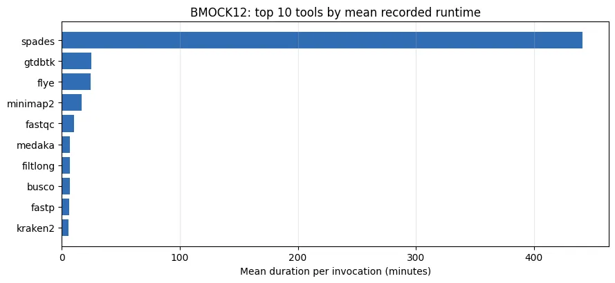

	mean_duration_min	n_runs
tool
spades	441.4	36
gtdbtk	24.8	36
flye	24.6	26
minimap2	16.7	72
fastqc	10.2	72
medaka	7.0	36
filtlong	6.9	36
busco	6.7	36
fastp	6.0	72
kraken2	5.6	216

5. Container images actually used (all three datasets)

The provenance records the exact container image for every step — the basis for re-running the workflow identically.

all_rows = pd.concat(worked.values(), ignore_index=True)
img = (
    all_rows["image"]
    .value_counts()
    .head(8)
    .rename_axis("container image")
    .reset_index(name="step invocations")
)
img

	container image	step invocations
0	docker-registry.wur.nl/m-unlock/docker/sapp:2.0	2284
1	quay.io/biocontainers/pigz:2.8	1785
2	quay.io/biocontainers/kraken2:2.1.3--pl5321hdcf5f25_0	648
3	docker-registry.wur.nl/m-unlock/docker/kofamscan:1.3.0-db.2024-01-01	571
4	docker-registry.wur.nl/m-unlock/docker/interproscan_v5:base	571
5	oschwengers/bakta:v1.9.4	479
6	quay.io/biocontainers/krakentools:1.2--pyh5e36f6f_0	324
7	quay.io/biocontainers/krona:2.8.1--pl5321hdfd78af_1	324

6. Functional annotation results (GBOL graph)

The second deposited query traverses the GBOL graph from samples to their functional annotations. The rows below use the final benchmark runs (BMOCK12 spades and flye-medaka configurations) and show, for each reconstructed MAG, the Pfam domains annotated by InterProScan.

pf = pfam[~pfam["sample_name"].str.contains("subset")].copy()
print("Final-run MAGs in the BMOCK12 Pfam table:", pf["sample_name"].nunique(), "| Pfam annotations:", len(pf))
per_mag = (
    pf.groupby("sample_name")["accession"]
    .nunique()
    .sort_values(ascending=False)
    .rename_axis("MAG")
    .reset_index(name="distinct Pfam domains")
)
per_mag.head(6)

Final-run MAGs in the BMOCK12 Pfam table: 45 | Pfam annotations: 97664

	MAG	distinct Pfam domains
0	BMOCK12_SRR_run_3_spades-medaka_rerun_SemiBin_11	2467
1	BMOCK12_SRR_run_1_spades-medaka_SemiBin_3	2445
2	BMOCK12_SRR_run_2_spades-medaka_SemiBin_8	2442
3	BMOCK12_SRR_run_3_spades-medaka_rerun_SemiBin_12	2440
4	BMOCK12_SRR_run_1_spades-medaka_MetaBAT2_bin.14	2426
5	BMOCK12_SRR_run_2_spades-medaka_MetaBAT2_bin.2	2426

print("Example rows (MAG -> Pfam domain; one spades and one flye-medaka bin):")
spades_ex = pf[pf["sample_name"].str.contains("spades-medaka")].head(3)
flye_ex = pf[pf["sample_name"].str.contains(r"BMOCK12__SRR_run_1_medaka_", regex=True)].head(3)
pd.concat([spades_ex, flye_ex])

Example rows (MAG -> Pfam domain; one spades and one flye-medaka bin):

	sample_name	accession
0	BMOCK12_SRR_run_1_spades-medaka_MaxBin2.bin.003	PF13692
1	BMOCK12_SRR_run_1_spades-medaka_MaxBin2.bin.003	PF10707
2	BMOCK12_SRR_run_1_spades-medaka_MaxBin2.bin.003	PF00535
72647	BMOCK12__SRR_run_1_medaka_MetaBAT2_bin.3	PF03976
72648	BMOCK12__SRR_run_1_medaka_MetaBAT2_bin.3	PF09424
72649	BMOCK12__SRR_run_1_medaka_MetaBAT2_bin.3	PF07859

7. Full provenance query (previously executed)

The deposited query templates also include a full version that adds the ISO-8601 duration and a human-readable step label. Example rows for the ZYMO-EVEN flye–medaka runs:

fullf = full[~full["input"].fillna("").str.contains("subset")].copy()
fullf["step"] = fullf["label"].str.extract(r"#main/([a-z0-9_]+)$")[0]
fullf[["step", "startTime", "endTime", "image", "duration", "input"]].head(5)

	step	startTime	endTime	image	duration	input
16	metaquast_medaka	2024-11-08T14:16:48.679415	2024-11-08T14:19:21.040005	docker-registry.wur.nl/m-unlock/docker/quast:5.2.0	P0Y0M0DT0H2M32.361S	NaN
17	metaquast_medaka	2024-11-08T14:16:48.679415	2024-11-08T14:19:21.040005	docker-registry.wur.nl/m-unlock/docker/quast:5.2.0	P0Y0M0DT0H2M32.361S	NaN
18	metaquast_medaka	2024-11-15T01:17:03.456572	2024-11-15T01:18:57.976545	docker-registry.wur.nl/m-unlock/docker/quast:5.2.0	P0Y0M0DT0H1M54.520S	NaN
19	metaquast_medaka	2024-11-15T01:17:03.456572	2024-11-15T01:18:57.976545	docker-registry.wur.nl/m-unlock/docker/quast:5.2.0	P0Y0M0DT0H1M54.520S	NaN
20	gtdbtk	2024-11-08T19:00:49.956975	2024-11-08T19:24:27.065377	quay.io/biocontainers/gtdbtk:2.4.0--pyhdfd78af_1	P0Y0M0DT0H23M37.109S	NaN

8. Biological interpretation — functional predictions across assembly configurations

The same FAIR functional-annotation framework supports a biological reading of the benchmark, not only an execution audit. The query below counts, per reconstructed MAG, the Pfam domains annotated by InterProScan in the GBOL graph; summing the counts per configuration and replicate run shows whether the predicted functional content is stable across runs or affected by the assembly/binning configuration.

PREFIX gbol: <http://gbol.life/0.1/>
PREFIX prov: <http://www.w3.org/ns/prov#>
SELECT ?sample (COUNT(?domain) AS ?nPfamDomains)
WHERE {
  GRAPH ?g {
    ?contig gbol:sample ?sample .
    ?contig gbol:feature/gbol:transcript/gbol:feature/
            gbol:protein/gbol:feature ?feature .
    ?feature gbol:provenance/gbol:origin/prov:wasAttributedTo
             <http://gbol.life/0.1/InterProScan/interpro> .
    ?feature gbol:accession ?domain .
    FILTER(STRSTARTS(STR(?domain), "PF"))
  }
}
GROUP BY ?sample

The table below is the archived result of this analysis (per configuration, the sum over all recovered bins of its three replicate runs; the GBOL graph itself contains the same data). The source column records which configurations are part of the public Zenodo functional-annotation graphs (public) and which are from the internally generated functional RDF that has not yet been published (internal).

pfam_cfg = pd.read_csv(RES / "bmock12_pfam_domains_per_config.csv")
label = {
    "spades_v2": "spades",
    "medaka_dtm": "flye-medaka (deterministic)",
    "medaka_pypolca": "flye-medaka-pypolca",
    "flye_pypolca": "flye-pypolca",
    "nondtm": "flye-medaka (non-deterministic)",
}
pfam_cfg["configuration"] = pfam_cfg["config"].map(label)
wide = pfam_cfg.pivot_table(
    index="configuration",
    columns="run",
    values="n_pfam_domains",
)
wide["range"] = wide.max(axis=1) - wide.min(axis=1)
src_by_cfg = pfam_cfg.groupby("config")["source"].first().to_dict()
label_to_cfg = {v: k for k, v in label.items()}
wide["source"] = wide.index.map(lambda c: src_by_cfg[label_to_cfg[c]])
wide

run	run_1	run_2	run_3	range	source
configuration
flye-medaka (deterministic)	37116.0	37114.0	37119.0	5.0	public
flye-medaka (non-deterministic)	36242.0	36545.0	37000.0	758.0	internal
flye-medaka-pypolca	48347.0	48364.0	48353.0	17.0	internal
flye-pypolca	49114.0	49110.0	49115.0	5.0	internal
spades	53652.0	53652.0	53652.0	0.0	public

fig, ax = plt.subplots(figsize=(9, 4.6))
x = range(len(wide))
width = 0.26
for i, run in enumerate(["run_1", "run_2", "run_3"]):
    ax.bar([p + (i - 1) * width for p in x], wide[run], width, label=run.replace("_", " "))
ax.set_xticks(list(x))
ax.set_xticklabels(wide.index, rotation=20, ha="right")
ax.set_ylabel("Total Pfam domain annotations")
ax.set_title("BMOCK12: predicted Pfam domains per configuration and replicate run")
ax.legend()
ax.grid(axis="y", alpha=0.3)
fig.tight_layout()
plt.show()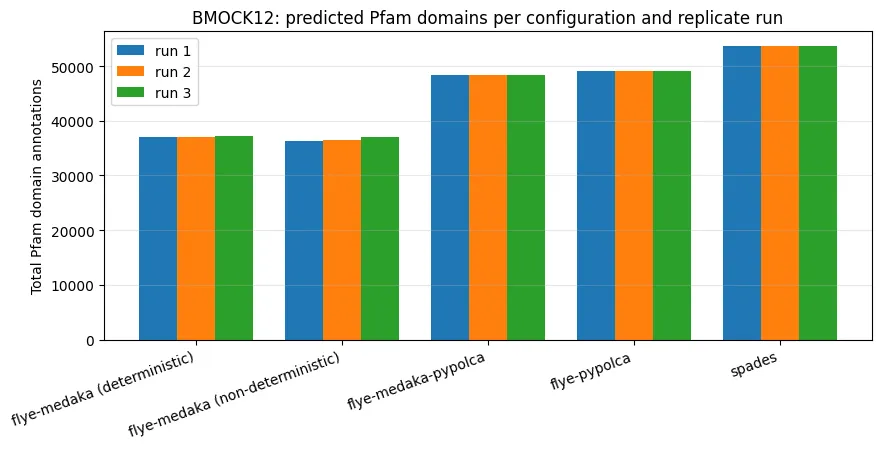

Reading the result

• spades (deterministic): 53,652 Pfam domain annotations in every replicate — functionally identical predictions across runs.
• flye-medaka (deterministic): 37,116 / 37,114 / 37,119 — effectively stable (residual differences of a few domains, consistent with stochastic binning steps).
• flye-medaka (non-deterministic): 36,242 → 36,545 → 37,000 — clear run-to-run drift, i.e. the non-deterministic configuration changes the predicted functional content between replicates.
• flye-pypolca / flye-medaka-pypolca: small run-to-run variation, intermediate between the deterministic and non-deterministic flye-medaka cases.

Interpretation. Non-deterministic assembly settings propagate to downstream functional predictions: the same data, analysed with the non-deterministic configuration, yields measurably different Pfam domain totals across replicates, while deterministic configurations are stable. This supports the manuscript’s conclusion that algorithmic determinism affects not only assembly contiguity but also biological interpretation.

Reference genomes (public reference_graph) provide species-level expectations, e.g. Cohaesibacter sp. ES.047 = 5,529 Pfam domains in the deposited graph (the value differs slightly from an independently re-annotated run because of the InterProScan version used; see manuscript discussion). Halomonas sp. HL-93 = 5,096 and HL-4 = 5,144.

Data-source note: public configurations (spades, deterministic flye-medaka, references) are retrievable from the deposited Zenodo functional-annotation graphs; the other configurations currently exist only in the internally generated functional RDF and are shown here to make the comparison complete.

9. Reproduce it yourself (optional)

This page is pre-rendered, so nothing needs to be run to read the results above. To reproduce them:

pip install pyoxigraph
python provenance_worked_example.py

The script downloads the three public provenance graphs from Zenodo and re-runs the query above, writing the same tables to results/. Expected run times on a laptop: ZYMO-LOG ~10 s, BMOCK12 ~2 min, ZYMO-EVEN ~9 min.

Resources

• Manuscript Methods: Worked provenance query
• Data: Zenodo 10.5281/zenodo.17990145
• Notebook & results: UNLOCK workflow analysis repository, branch demo/provenance-worked-example
• FAIR Data Station documentation: fairbydesign.nl/docs